PyTamaro is based on a principled foundation: algebra. The reasoning about PyTamaro graphics corresponds to the reasoning about algebraic expressions.

Graphics are Immutable

Our approach to programming with graphics can work like algebra only because it avoids mutable state.

Once we have a graphic, we cannot modify it! There is no way to, e.g., change the rotation angle of a graphic.

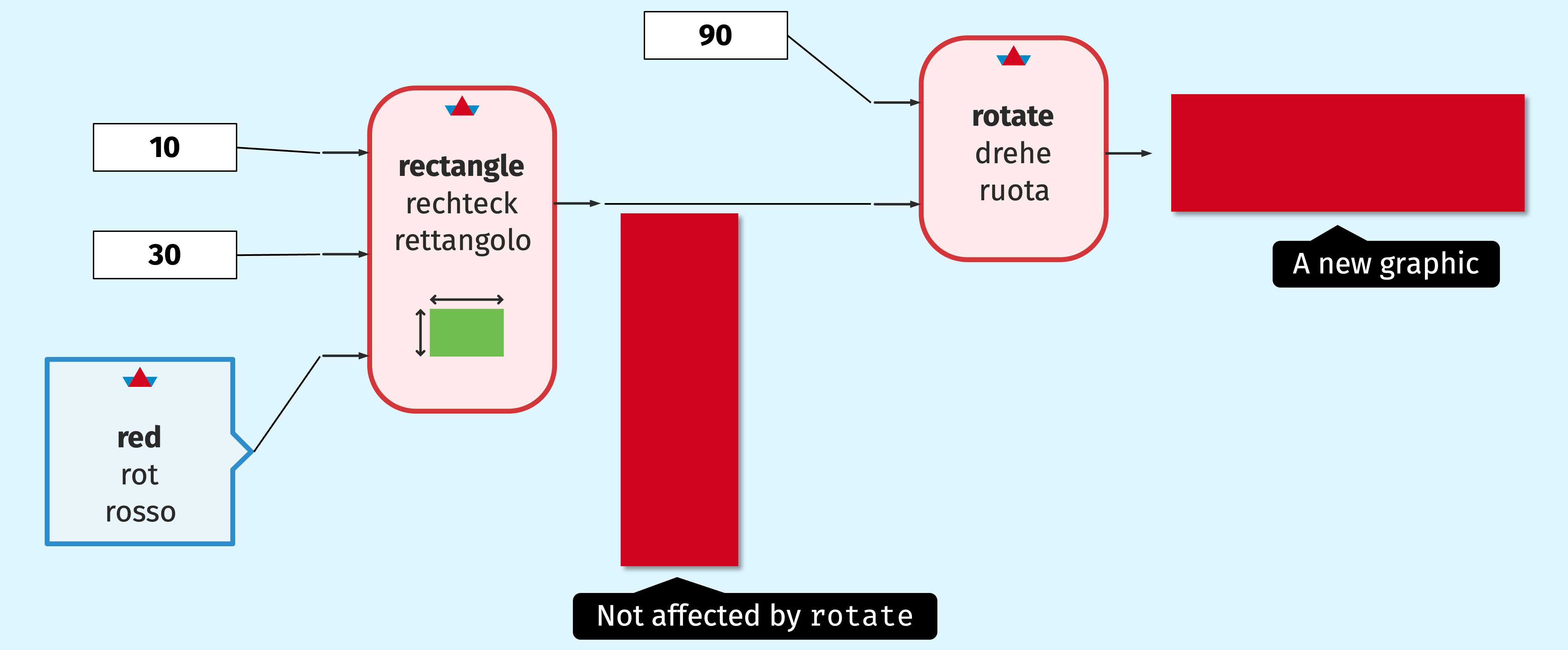
Run the following code, and observe how the graphic the name stick refers to will not be affected by the call of rotate (rotate will not mutate the graphic).

What rotate does is to produce a new graphic, that is a rotated copy of the original. Check this out:

The first line creates a vertical rectangle. The second line creates a rotated copy (a horizontal rectangle) and shows that. The last line shows the original, unmodified vertical rectangle.

Functions are Pure

PyTamaro functions like rectangle and rotate are pure: they always produce the same result value for given argument values, no matter how many times, when, or from where you call them.

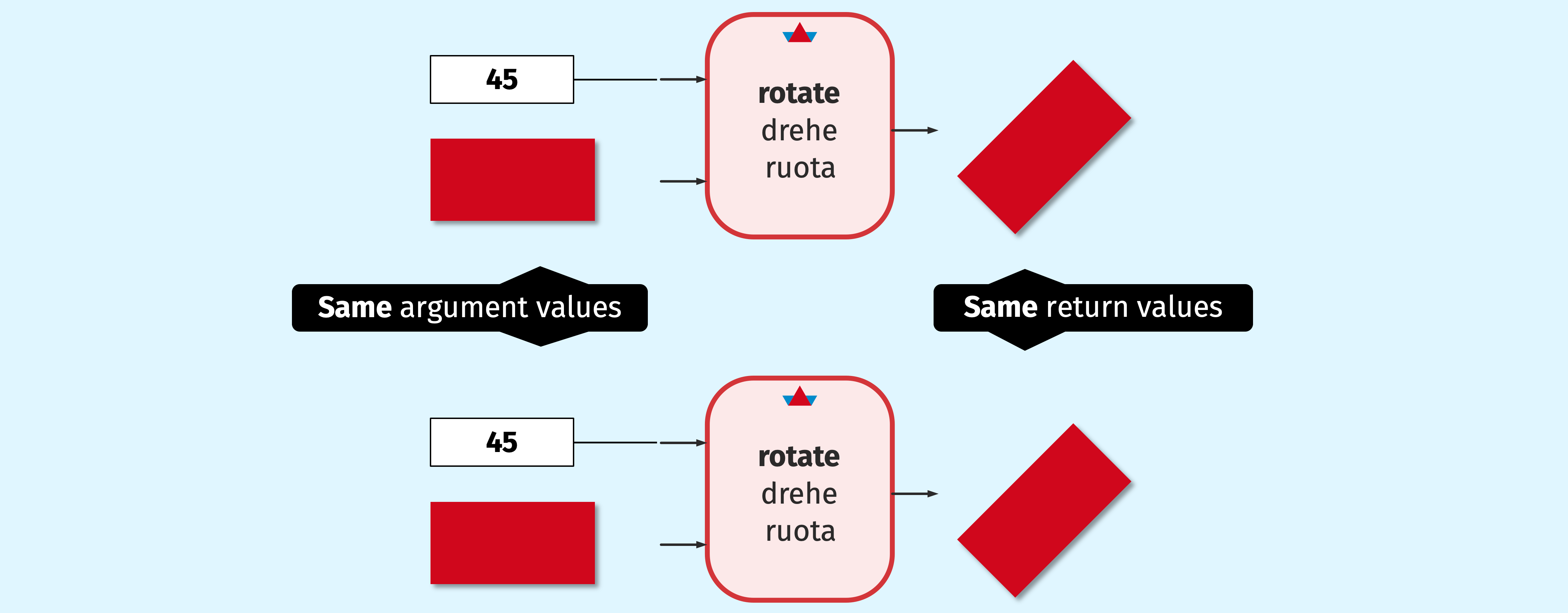
Give it a try:

This will show three times the exact same rectangle. This seems quite desirable, right?

A Set Of Values

The type Graphic represents the set of all possible graphics (any kind of rectangle, ellipse, circular sector, and any arbitrarily complex composition of those).

This is similar to the set ℝ of real numbers in math, which corresponds to all possible numbers.

In math we have many different real number values, such as 0, 0.5, 1000, and -2.

In PyTamaro, we have many different graphic values that can be produced by calling functions such as rectangle and ellipse.

A Binary Operation for Composition

In elementary algebra, we have the plus operator, with which we can compose a new number out of two existing numbers:

In PyTamaro, we have the compose function, with which we can compose a new graphic out of two existing graphics:

That Operation is Associative

Note that both, the arithmetic + operator and the compose function are associative. Here is what this means:

Let's look at an example:

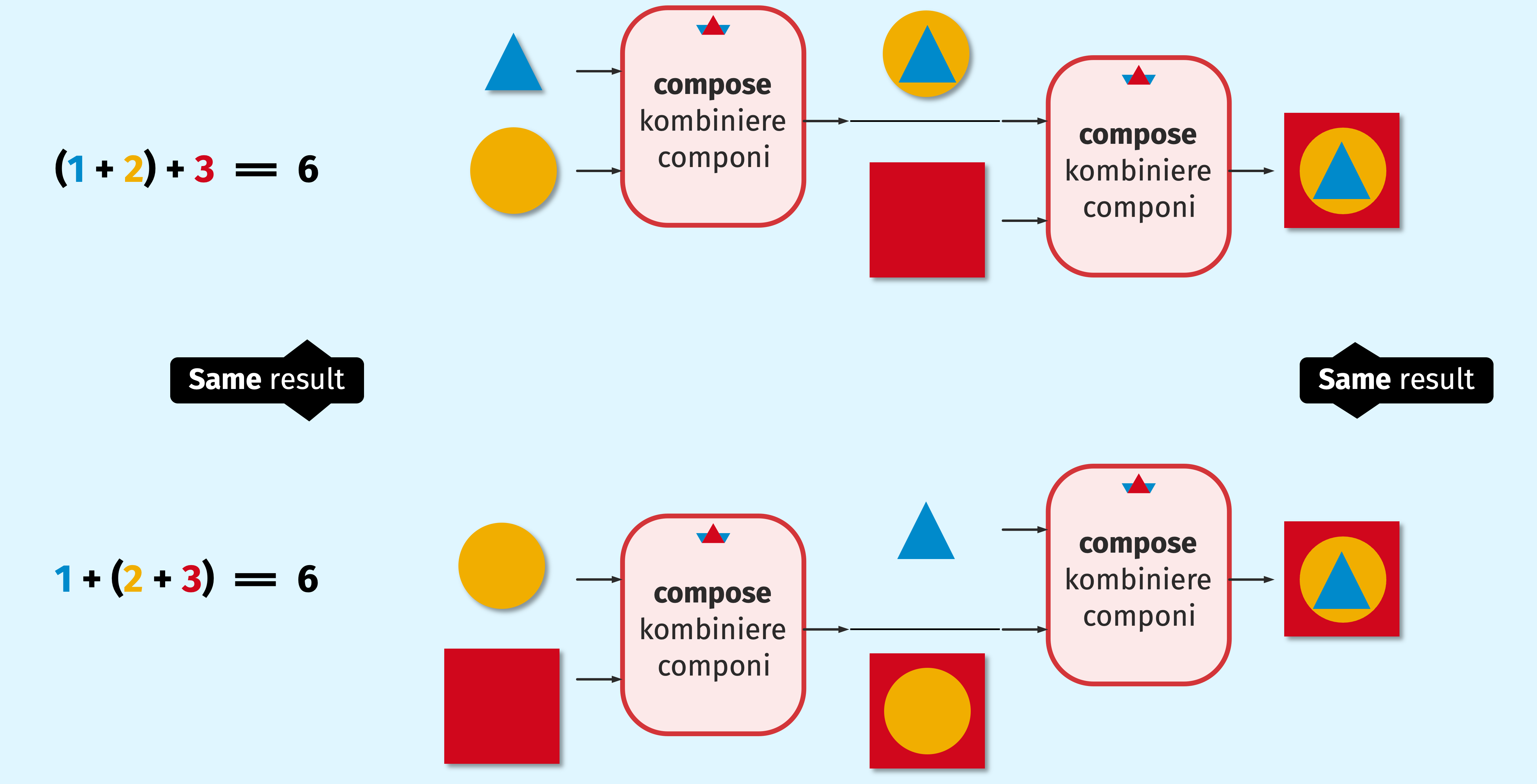
Let's try this out! The following pairs of statements should produce the same outputs:

The same applies to compose. Both of the following statements should output the same graphic:

A Semigroup

If we have a set of elements and an associative binary operation on that set, abstract algebra calls that a semigroup.

Both, the real numbers with the + operator, and the PyTamaro graphics with the compose function, are such semigroups.

An Identity Element

In elementary algebra, the number 0 is quite a special value: it serves as the identity element of addition. In PyTamaro graphics, the result of calling empty_graphic is an equally special value: it serves as the identity element of compose. Let's see what that means:

Here is an example:

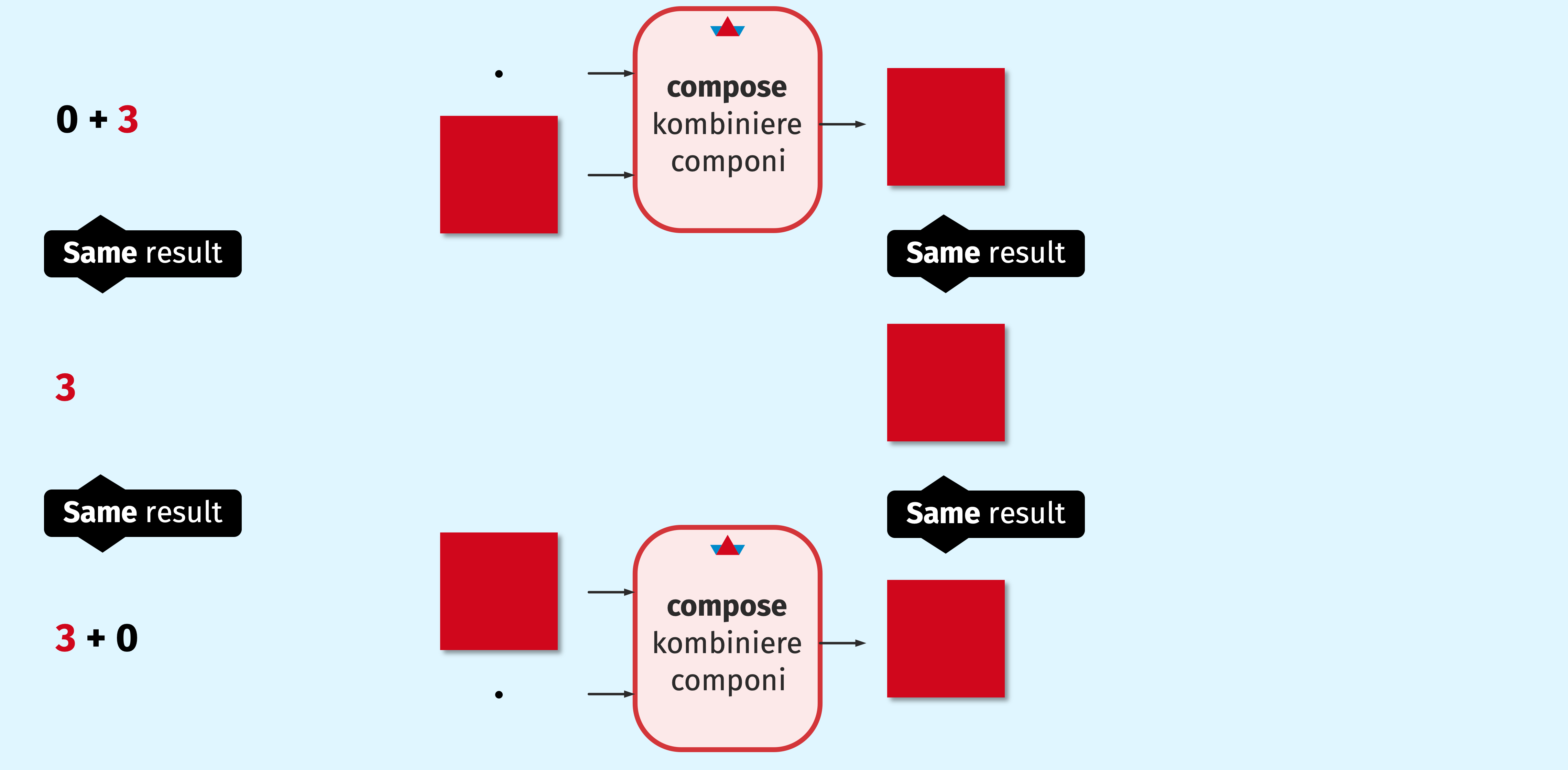
Because 0 is the identity element of addition, the following three statements all produce the same output:

Similarly, the following three statements all produce the same output:

A Monoid

Once we have a semigroup and an identity element, we have an algebraic structure called a monoid.

Both, the real numbers with the + operator and the identity element 0, and the PyTamaro graphics with the compose function and the identity element empty_graphic(), are such monoids.

Monoids Enable Decomposing Reductions

Why do we care about something as exotic as a monoid? Well, monoids can help us to write efficient parallel and distributed computations. How? They are at the heart of a kind of repetitive computation called reductions. Reductions compose multiple values into some aggregate. Here are a few examples:

• Sum a list of values
• Place all the graphics in a list beside each other
• Find the minimum, maximum, or arithmetic mean of a list of numbers
• Compute the conjunction over a list of Booleans
• Join together a list of strings

Here is an example. A function that reduces a list of numbers into their sum:

And here is an example graphic composition:

Both these examples wouldn't require a monoid: they work also if the binary operation is not associative.

Where the associativity provided by the monoid becomes helpful is when we want to break a longer reduction (say, of millions or billions of elements) onto multiple independent subtasks that could be executed in parallel, on different processors or different computers (say, reduce the first million elements on computer A, and at the same time reduce the second million on computer B, and then combine the results of the two reductions by reducing them, too).

The ability to decompose such a reduction into multiple independent reductions can provide large performance gains, especially in todays world where processors have many cores, and computation happens across clusters of computers.

A Unary Operation

In elementary algebra, we know the unary minus operator. It takes a single number and negates it:

In PyTamaro, we have a function named rotate that takes a single graphic and rotates it:

Our rotate function also takes the number of degrees by which that graphic is to be rotated. We could, however, easily create our own variant of rotate, that takes only a single argument, the graphic, and always rotates that by a specific angle:

A Monoid Endomorphism

The unary operation, on an element of a monoid, is called a monoid endomorphism under the given operation of the monoid, if the following conditions hold:

Here is an example:

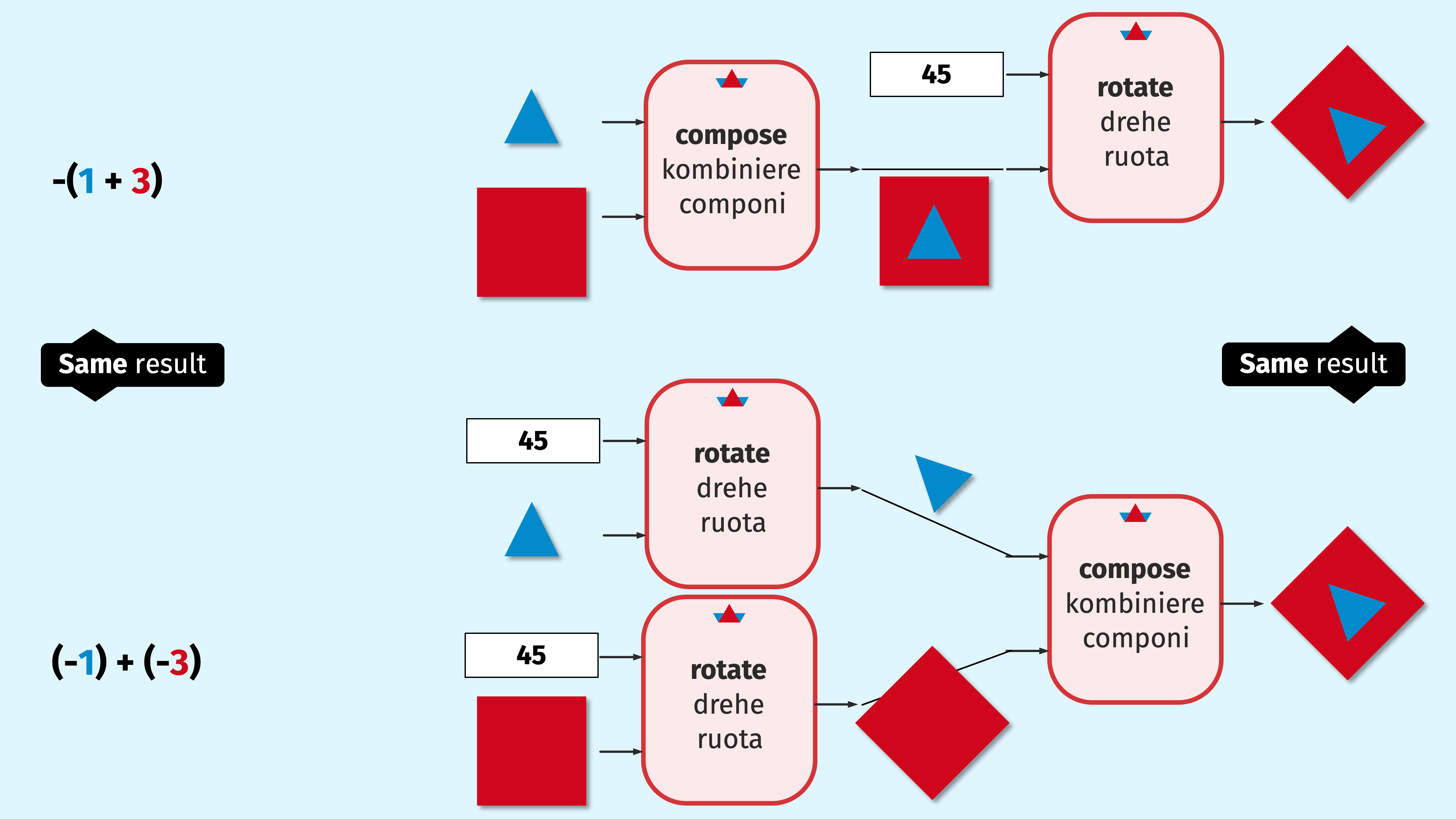
Play with the example in the following code cell (check whether the results are the same for numbers other than 1 and 3):

Similarly, play with the rotation of graphics (check whether the results are the same for graphics other than tri and box):

Conclusion

We have seen quite a few algebraic concepts and how they manifest themselves in school algebra as well as PyTamaro graphics. Let's look at a tabular summary:

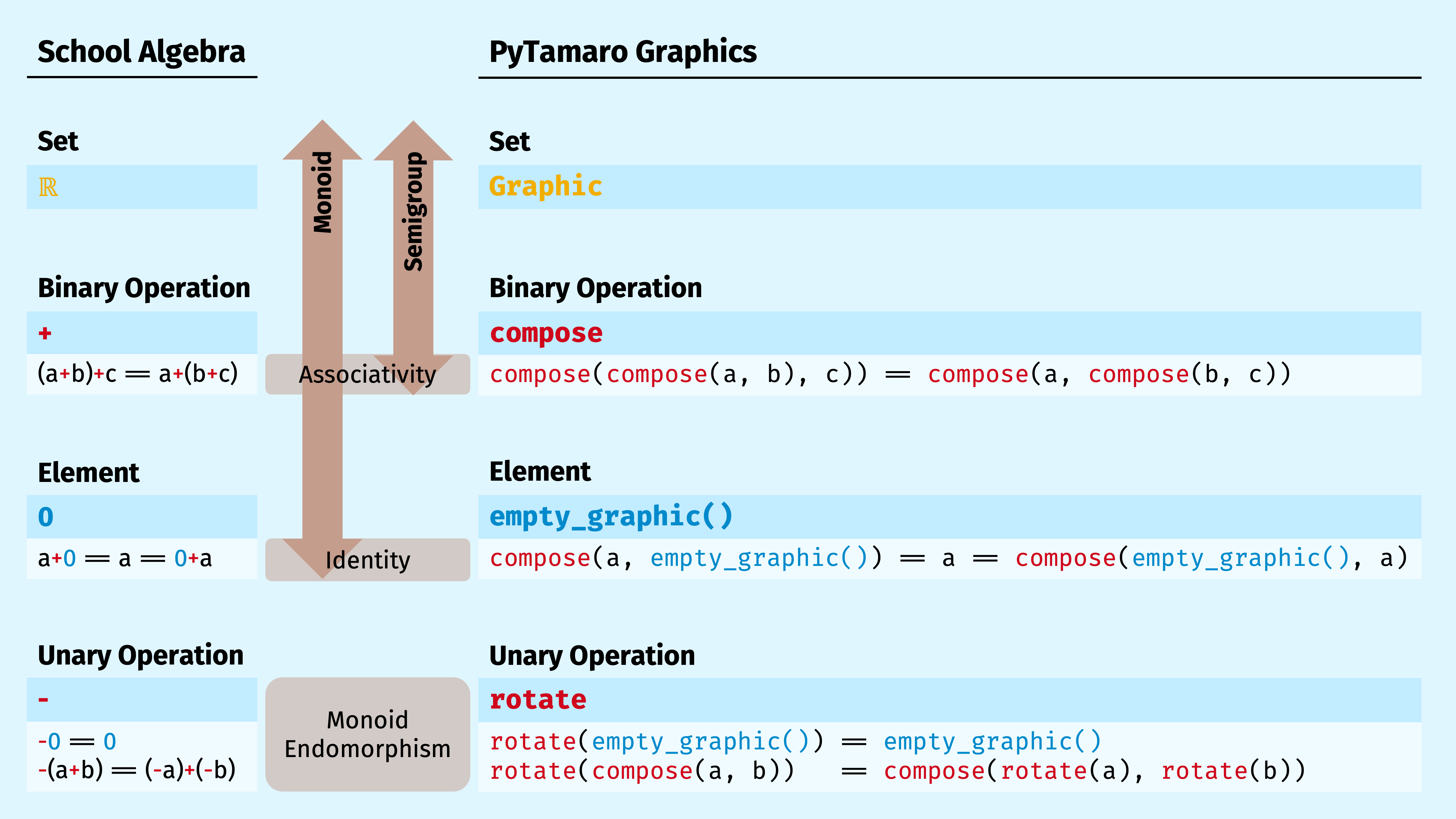
We discussed sets of values and associative binary operations on such sets, which together form what abstract algebra calls semigroups. Then we discussed identity elements, which together with a semigroup form a monoid. Finally, we discussed monoid endomorphisms.

We can reason about elementary algebra expressions in exactly the same way as we can reason about PyTamaro graphics expressions. We can use the properties in the table to rewrite and simplify expressions.

This is no coincidence: PyTamaro is a pure functional library (with pure functions and immutable values), and pure functional programming is essentially just algebra: a bunch of sets, values, and operations, and a few laws we can use to rewrite expressions to simplify them or reduce them to a value.

Beyond Algebra

Of course Python, the programming language we use, is not limited to pure functions and immutable values.

One can easily use or define an impure function. In fact, our show_graphic function is impure (click on it here to see the explosion icon we use in the API documentation to indicate that a function is impure), as is Python's built in print function.

In Python one also can easily mutate variables. It is up to the educator to decide when in a curriculum to introduce mutation of variables. It can be best to initially not even mention mutable variables, but to just talk about "names" or "constants". Students who never programmed before (but have studied arithmetic and elementary algebra for many years), may not come up with the—for them—somewhat strange idea of mutable variables.

Note that as soon as one uses mutation and impure functions, we can't rely on the nice algebraic properties anymore; we move from pure functional programming, with a "substitution semantics" like in algebra, to imperative programming, with a more complex semantics that requires a model of mutable state.

However, not all is lost: One can keep most of the functions pure, and only resort to impurity where truly needed (e.g., for input and output). And one can refrain from using mutable state in many situations, and for example limit the use of mutable variables to specific situations within functions. This is a general design principle for good professional programmers.

Learning More

If you want to learn more about the deep connections between programming and math, and about functional programming, check out a language like Haskell, the Racket Student Languages, or Scala, or have a look at our Masters course on Programming Styles, where we show these basic as well as more advanced functional programming ideas in traditional imperative programming languages like Java.